Qiskit2.0 : Your Fast-track Start Guide

1. What You’ll Learn

• Quickly understand the major improvements and new features introduced in Qiskit 2.0 / 2.1

• Run quantum experiments locally with up to approximately 20 qubits using simulators like AerSimulator, StatevectorSampler, and StatevectorEstimator

• Hands-on experience covering Fake Backend → Real Quantum Hardware → AI-assisted Transpilation → Session Mode

• Clear overview of IBM Quantum Plans, from Open to Premium and Flex

• Practical steps, including API key storage, job management, and result analysis

2. Who This Guide is For

• Quantum Computing Beginners: no advanced terminology required

• Programming Beginners: Basic Python skills are enough

• Hands-On Learners: Learn by actually running code!

3. About Us

The SoftBank Research Institute of Advanced Technology was established in 2022. In 2023, we launched our Quantum Technology Development Division, actively conducting experiments with real quantum hardware from IBM and Quantinuum. Our team includes experts in quantum error correction, quantum chemistry, quantum machine learning, quantum optimization, and quantum communication.

4. Recommended Setup

The Japanese-specialized large language model ”Sarashina mini”, developed by SB Intuitions[2], achieves highly accurate Japanese text generation.[3]
Choosing a stable OS and Python combination helps avoid potential issues from the start!

[1] Sarashina Chat – Latest Updates
https://notes.sarashina.sbintuitions.com/

[2] SB Intuitions Corp.
https://www.sbintuitions.co.jp/
[3] SoftBank Corp. – Press Release
https://www.softbank.jp/corp/news/press/sbkk/2025/20250723_01/

5. What’s New in Qiskit 2.x[4]

In 2025, Qiskit has officially moved into its 2.x era. While the overall direction from the 1.x series remains, this new release brings a host of improvements that make life easier for quantum developers. Let’s walk through the highlights.

A Simpler Package Structure

With Qiskit 2.x, you only need to install the Qiskit metapackage—everything you need comes bundled in one place. You no longer have to manage qiskit-terra or qiskit-aer separately, which means fewer headaches with dependencies.

Stable, Compatible APIs

Qiskit 2.x follows semantic versioning, giving developers confidence about compatibility:

• Major versions (2.x → 3.x): may include breaking changes

• Minor versions (2.1 → 2.2): introduce new features

• Patch versions (2.1.0 → 2.1.1): fix bugs

This makes it easier to plan long-term projects without fear of sudden disruptions.

Faster with Rust

Parts of the transpiler have been rewritten in Rust, delivering around 20% performance improvements. For researchers handling large circuits, this is a significant speed boost.

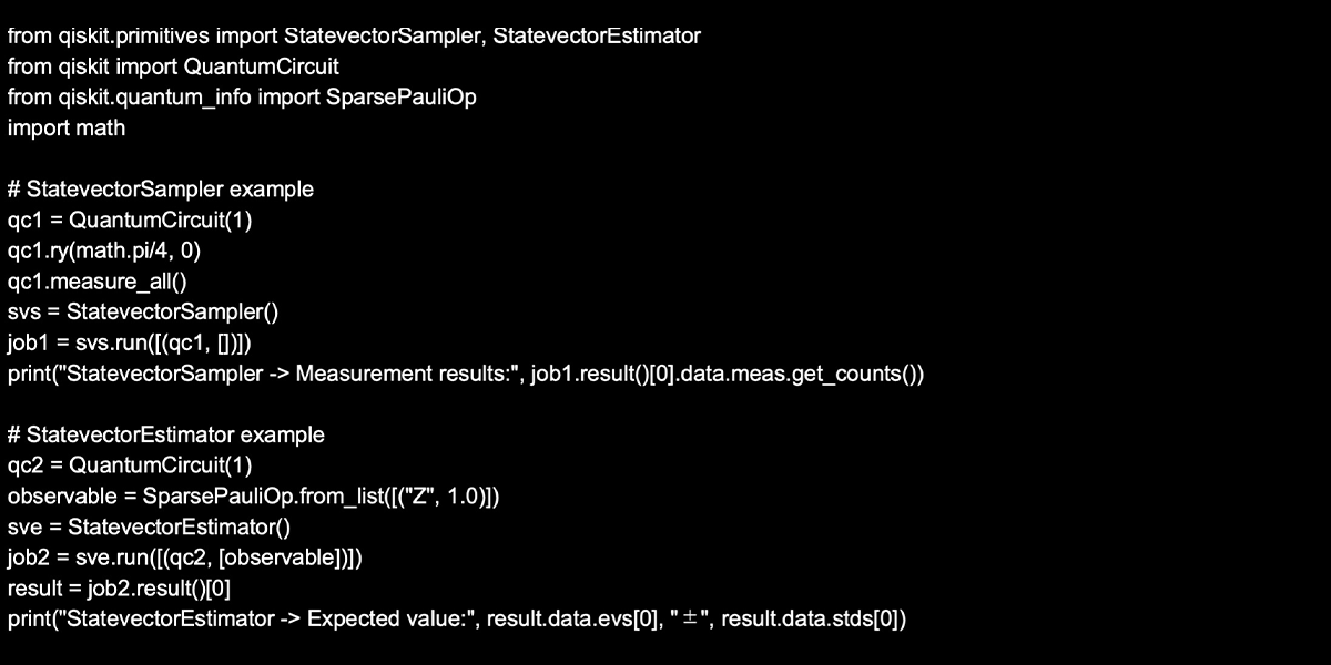
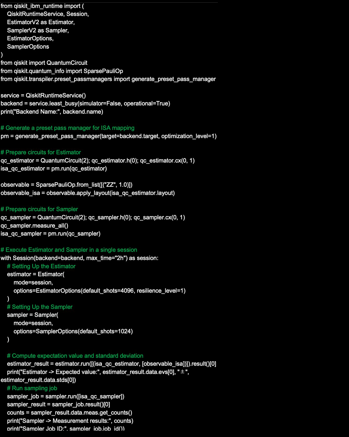
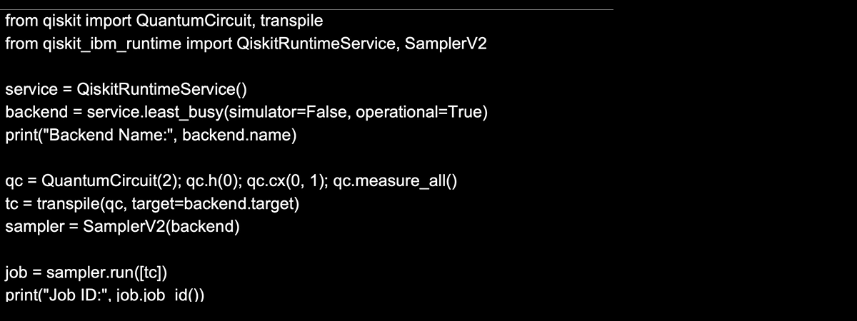
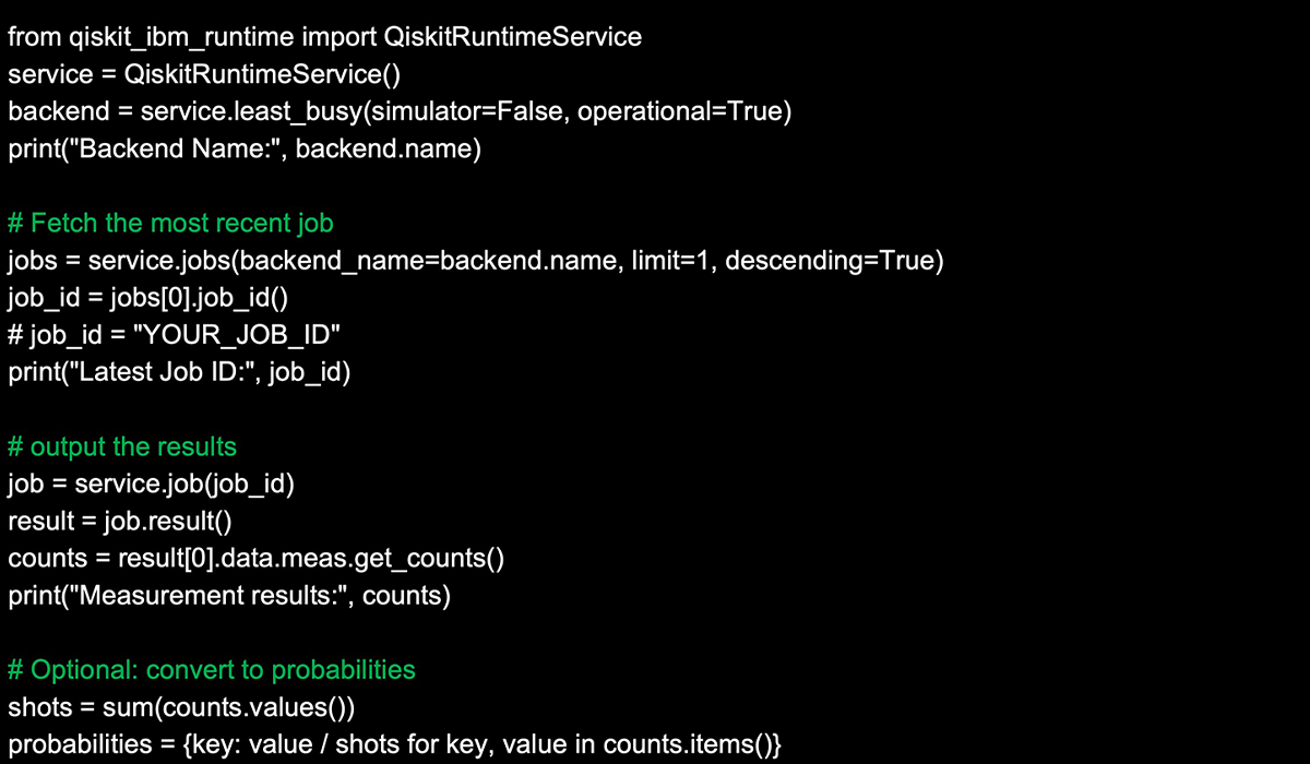
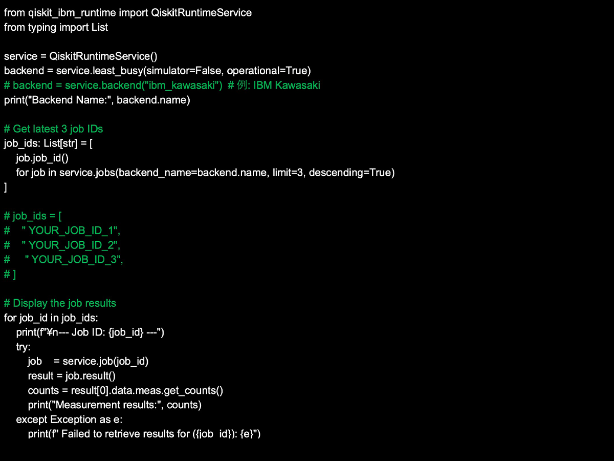
Smarter Primitives API

The Primitives API—the building blocks of quantum computing—has been expanded with more flexible input and output options. This makes it easier to design and customize experiments.

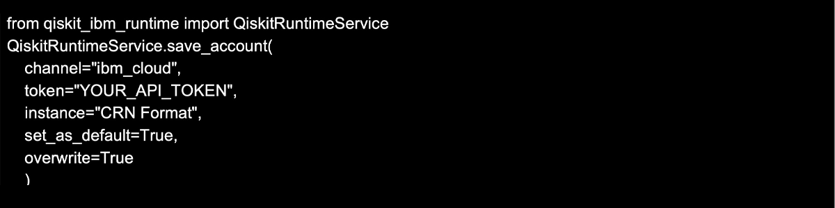
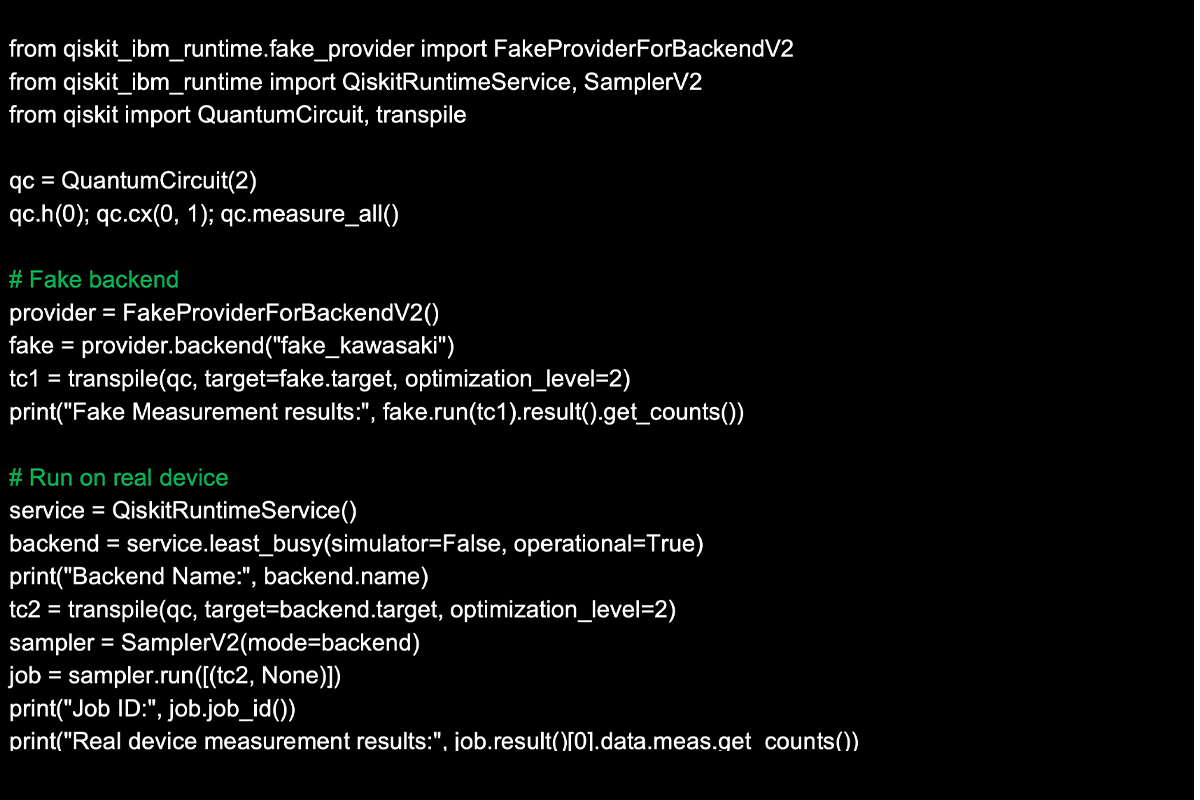
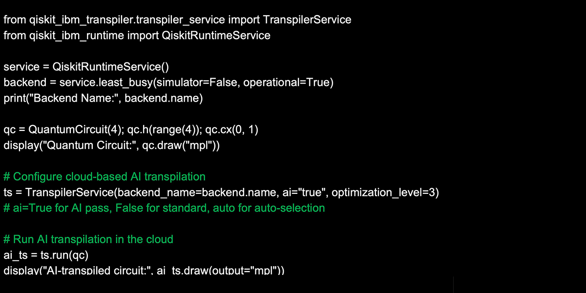
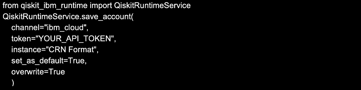
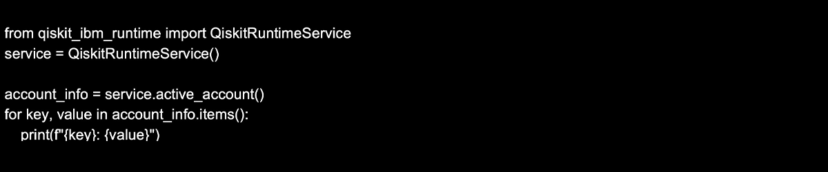
Expanded Authentication and Services

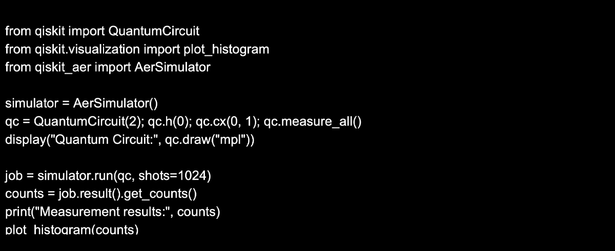
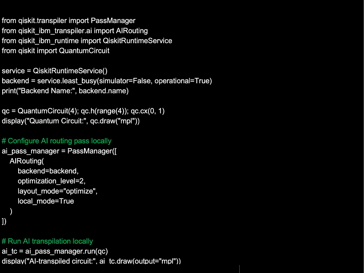
Cloud integration has become more flexible, with multiple authentication channels now available. A new local mode also lets you run primitives (like Sampler and Estimator) directly on local simulators such as AerSimulator.

• ibm-quantum-platform – the newest channel, used by default in modern Qiskit Runtime

• ibm-cloud – still available, but gradually being replaced by ibm_quantum_platform

• ibm-quantum – deprecated and removed in recent Runtime versions (e.g., v0.40.0+)

• Local – for running primitives on your own machine with simulators

More Powerful Simulator API

The simulator API has been upgraded with better performance and richer options, making trial-and-error experimentation much smoother.

Stronger OpenQASM Support

Control flow in OpenQASM has been enhanced, allowing for more expressive circuit descriptions.

C/C++ API Support

Until now, Qiskit was primarily Python-based. With 2.x, developers can now use C and C++ to build circuits, configure targets, and even work with new features like SparseObservable. Integration between C and Python is also supported.

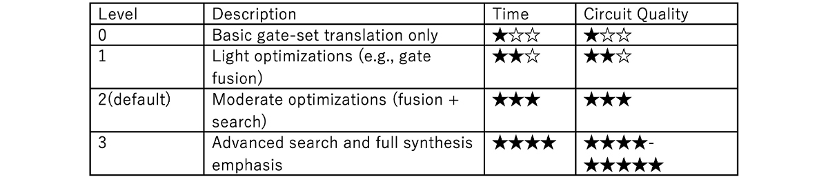
Smarter Transpilation Optimizations

If your circuit is expressed in the Clifford+T basis, Qiskit automatically applies optimized transpilation paths, delivering faster results with hardware-friendly circuits.

Python 3.9 Deprecated

One note of caution: starting from Qiskit 2.3, Python 3.9 is no longer supported. You’ll need Python 3.10 or later.

Wrapping Up

Qiskit 2.x represents an evolution that keeps ease of use while boosting performance and flexibility. From Rust-based acceleration to C/C++ support, it’s designed to widen the scope of who can work with quantum computing.
Whether you’re just getting started or already deep into development, the latest Qiskit is worth exploring.

[4] Qiskit 2.0 Release Summary（IBM Quantum Blog）
https://www.ibm.com/quantum/blog/qiskit-2-0-release-summary

6. Environment Setup Steps

Let’s get your environment up and running.

1. Create a Virtual Environment

Open your terminal and run
$bash

You should see (.venv) in your prompt.

To deactivate the environment, run
$bash

2. Install Required Packages in Jupyter Notebook

In a notebook cell, run

Installing packages directly in the cell lets you prepare the environment on the spot!

3. Check Your Python Version

Python 3.11 or 3.12 is recommended.

[5] Introduction to Qiskit
https://quantum.cloud.ibm.com/docs/en/guides

7. From Simulator to Real Hardware: How to Run Quantum Circuits

At this point, you should have your Qiskit 2.x environment up and running.
So, what’s next? It’s time to take a closer look at how to actually execute a quantum circuit.

When working with quantum computers, the workflow generally follows these three steps:

1. Primitive APIs (explained in Chapter 8)

The starting point is the Primitive APIs—interfaces like the Sampler and Estimator.
Think of these as the “gateways” for running quantum calculations.
The beauty here is consistency: whether you’re working locally (e.g., with statevectors) or on real hardware via the cloud, you use the same interface.

2. Simulation (explained in Chapter 9)

Before sending your circuit to real quantum hardware, you’ll want to test it on your PC first.
This can be a noise-free “ideal experiment” using a statevector simulator, or a more realistic one using AerSimulator, which mimics hardware noise.
In short: simulation helps confirm that your circuit behaves as expected before you take the next step.

3. Real Quantum Hardware (Fake Backend → IBM Quantum Platform, explained in Chapter 10)

Once your circuit passes simulation checks, you can move closer to the real experience:
Start with the Fake Backend, which mimics the behavior of actual devices.
Then, when you’re confident, submit your job to a real IBM Quantum computer.

In Chapters 8–10, we’ll explore these three pillars—Primitives API, Simulators, and Real Quantum Hardware.
They aren’t separate silos, but rather parts of a workflow that naturally fit together:

1. Primitives API – a common interface for both simulators and hardware.
2. Simulators – your first stop to validate circuit behavior safely.
3. Real quantum hardware – the final step, running circuits on quantum computers to capture results with noise.

By cycling through these steps, we can safely implement and verify quantum algorithms.

This staged approach helps minimize issues while building practical experience.
From the next chapter onward, we’ll follow this flow step by step: Primitives API → Simulation → Real Quantum Hardware.

8. Primitives API[6]

Running Quantum Circuits in Qiskit 2.x: Simulators, Primitives, and Real Quantum Hardware.
When working with Qiskit 2.x, there are three main ways to run your quantum circuits:
1. Simulators
2. Primitives API
3. Real quantum hardware

These aren’t isolated options—you can choose depending on your goal, or even step up from one to another as your project evolves. Let’s break down how each path works and why you might choose one over the others.

Choosing Your Starting Point

If you just want to run quantum circuits and understand the basics:

The simplest option is to use a simulator directly, such as AerSimulator. This gives you quick, intuitive results.

If you want a smooth transition from “local testing → real hardware”:

Start with the Primitives API (Sampler / Estimator) and use them with a simulator. Later, when you switch to a real device, your code remains the same—you simply change the backend.

So the question becomes: Do you want a quick hands-on experience, or do you want to build with real hardware in mind?

What are the Primitives?
The Primitives API provides two core functions for quantum computation:

Estimator – Calculates the expectation value of a quantum circuit (returns averages and error margins).

Sampler – Runs a quantum circuit multiple times to obtain a probability distribution of measurement outcomes.

And depending on where you run them, there are two flavors:

Local versions (StatevectorSampler / StatevectorEstimator):

Run on your PC to get ideal, noise-free results. Good up to ~20 qubits.

Cloud versions (SamplerV2 / EstimatorV2):

Run on IBM’s cloud platform, connecting you to real quantum devices or high-performance simulators. Includes noise and error mitigation options.

The Big Picture

In short, the Primitives API acts as the gateway for running quantum computations. Whether you’re on a simulator or real hardware, you interact with your circuit through the same unified interface. That consistency makes it easier to scale your workflow from simple experiments to real-world execution.

[6] Primitives
https://quantum.cloud.ibm.com/docs/en/api/qiskit/primitives

9. Learn with Simulator!

Before jumping straight into a real quantum computer, it’s a good idea to start with a simulator—a safe local environment where you can test quantum circuits without risk.
Simulators provide an ideal, noise-free setting to check how your circuits behave. This makes them perfect for beginners who are learning the basics, as well as for debugging algorithms before running them on actual hardware.

When combined with the Primitives API, simulators also serve as a stepping stone toward seamless execution on real quantum devices. In other words, the same code you test locally can often be transferred directly to hardware later.

Think of it like a flight simulator for quantum computing. Just as pilots practice on a simulator before flying a real plane, you can rehearse your quantum circuits locally to confirm that everything works as intended—before taking off on a real machine.

In this section, we’ll explore hands-on experiments using tools like AerSimulator, StatevectorSampler, and StatevectorEstimator.

1. AerSimulator: lightweight probabilistic simulator

AerSimulator is lightweight and fast—perfect for initial experiments on larger circuits.

2. StatevectorSampler／StatevectorEstimator. full statevector computation (up to ~20 qubits)

These local simulators let you validate circuit behavior on up to 20 qubits before running on real hardware—great for confidence-building and debugging.

[7] Simulators
https://qiskit.github.io/qiskit-aer/tutorials/1_aersimulator.html>

[8] StatevectorSampler
https://quantum.cloud.ibm.com/docs/en/api/qiskit/qiskit.primitives.StatevectorSampler

[9] StatevectorEstimator
https://quantum.cloud.ibm.com/docs/en/api/qiskit/qiskit.primitives.StatevectorEstimator

10. Let’s Experience Real Quantum Hardware!

Important

Stepping Up to a Real Quantum Computer

After experimenting with simulators, the next big step is finally running your circuits on a real quantum computer.

But unlike simulators, actual devices come with unavoidable real-world limitations—noise, connectivity restrictions, and queueing delays. That’s why it’s best to take a gradual approach: first test your code on a Fake Backend, and then move on to an actual device on the IBM Quantum Platform.

The good news? If you’re using the Primitives API, most of your code can be reused with little or no change.

Fake Backend – Your Quantum “Mock Exam”

The Fake Backend is a testing environment that mimics the noise and hardware constraints of a real device.
It won’t give you perfect, “clean” results like a simulator—it deliberately introduces imperfections, so your outputs feel closer to what you’d expect from real hardware.

Think of it as a mock exam before the actual test. It prepares you for the quirks of quantum devices without the costs and waiting times of real execution.

IBM Quantum Platform – The Real Thing

Once you’re ready, you can connect to an actual quantum processing unit (QPU) on the IBM Quantum Platform. All you need is your API key to authenticate.

• Queueing delays – because many users are sharing the same devices.

• Noise – errors from imperfect qubits and gates.

• Connectivity constraints – not every qubit can talk directly to every other qubit.

Running your circuit here is the closest thing to a real-world quantum computing experience. At this stage, you’ve crossed from “practice” into the territory of research and practical applications.

Start with a simulator → move to a Fake Backend → graduate to a real QPU.
This step-by-step path makes your journey into quantum computing smoother—and much less frustrating.

1. Save your API token

Once saved, you can simply use `service = QiskitRuntimeService()` next time.
The credentials are stored in plain text, so avoid using shared machines.

2. From FakeBackend to Real Quantum Hardware

The FakeBackend gives noise-free results, while real hardware introduces noise, connectivity constraints, and queuing delays for an authentic experience!

[10] Set up your IBM Cloud account
https://quantum.cloud.ibm.com/docs/en/guides/cloud-setup

[11] Fake Provider
https://quantum.cloud.ibm.com/docs/en/api/qiskit-ibm-runtime/fake-provider

[12] Migrate to the Qiskit Runtime V2 primitives
https://quantum.cloud.ibm.com/docs/en/migration-guides/v2-primitives

11. Transpiler Optimization Levels[13]

Why Quantum Circuits Need Transpilation in Qiskit

When you design a quantum circuit in Qiskit 2.0, you can’t just run it directly on a real quantum computer.
The reason is simple: each quantum computer comes with its own set of available gates and hardware constraints (topology).
Even among IBM’s quantum computers, each device (or QPU chip) comes with a different number of qubits and unique connectivity between them. That means the same circuit may or may not be directly executable depending on the machine.

To solve this, Qiskit introduces a crucial step called transpilation—a process that rewrites and optimizes your quantum circuit so it fits the constraints of the specific backend (whether that’s a simulator or real quantum hardware).

What Happens During Transpilation?

Transpilation in Qiskit mainly involves two processes:

1. Gate Set Conversion

The circuit you create is rewritten using the basis gates supported by the target backend.
For example, even if you write your circuit with high-level gates, transpilation ensures they are broken down into the primitive operations that the hardware actually understands.

2. Optimization

The transpiler removes unnecessary gates, reduces circuit depth, and restructures operations to minimize the effect of noise and errors.

This optimization can be tuned using something called the optimization level (0–3):

• Level 0: Minimal changes, mainly just converting gates to the supported set

• Level 1: Basic optimizations, removing some redundant operations.

• Level 2: More aggressive optimizations, focusing on circuit depth and efficiency.

• Level 3: The most thorough optimization, exploring multiple possibilities to find the most efficient circuit (though this takes longer to compute).

In short, higher optimization levels often give you better results—but at the cost of longer transpilation time. Choosing the right level depends on your experiment’s scale and purpose.

Takeaway
Transpilation is what makes your carefully written quantum circuit actually runnable on real hardware.
By understanding gate set conversion and optimization levels, you can strike the right balance between speed and accuracy—tailoring your workflow to the quantum device at hand.

Normally, Level 2 (Standard) offers the best balance and is generally recommended.

• If you want to test things quickly → Level 0 or 1 works best.

• If you’re running research experiments where precision is critical → Level 3 is the way to go.

Choosing the right level for the right situation makes your workflow much more effective.

[13] Set transpiler optimization level
https://quantum.cloud.ibm.com/docs/en/guides/set-optimization

12. Experience AI-Based Transpilation & Cloud AI Passes!

Smarter Quantum Circuit Optimization with AI Transpilation in Qiskit 2.x

In Chapter 11, we talked about transpilation—the process of optimizing a quantum circuit before running it on real hardware. Traditionally, this step has relied heavily on search algorithms and heuristics, which worked but had their limits.

With Qiskit 2.x, things get a big upgrade: AI-powered transpilation (AI Pass). By incorporating machine learning, Qiskit can now deliver more efficient and higher-quality circuit optimizations than ever before.

What Makes AI Transpilation Different?
Here are the key points:

Machine learning models at the core

AI learns from past optimization data and the noise characteristics of real quantum hardware. This allows it to reduce circuit depth and gate count more effectively.

Two modes: Local and Cloud

• Local AI Transpilation

• Runs entirely on your PC, free and easy to try.

Best suited for small circuits or quick, iterative experiments.

• Cloud AI Transpilation

Available with an IBM Premium plan.
Uses cloud-based resources, making it powerful for large-scale circuit optimization.

Why Does This Matter for Users?

• Better performance on real hardware: fewer errors and shorter execution times.

• Higher throughput and accuracy without manually fine-tuning complex optimization settings.

• Hands-off optimization: instead of tweaking levels by hand, you can simply let the AI handle it.

In short, Qiskit has evolved beyond just choosing an “optimization level.” With AI, your circuits benefit from data-driven insights and automatic improvements.

What’s Next?
From here, we’ll take a closer look at both Local AI Transpilation and Cloud AI Transpilation, and see how they perform in practice.

Local Mode vs. Cloud Mode

• Local Mode (local_mode=True): Run AI-driven optimization passes on your machine—no internet or subscription required, allowing fast iteration.

• Cloud Mode (using TranspilerService with ai="true", etc.): Utilize a Premium Plan API token to offload heavy optimizations to IBM Cloud resources, scaling efficiently to large circuits.

1. Local AI Transpilation

AI passes can significantly reduce circuit depth and CNOT count!

2. Cloud AI Transpilation (Premium Plan only) [15]

Achieve even higher performance with cloud AI passes!

[14] qiskit_ibm_transpiler
https://github.com/Qiskit/qiskit-ibm-transpiler

[15] PyPi qiskit-ibm-transpiler
https://pypi.org/project/qiskit-ibm-transpiler/

13. Session Mode (Available for Premium Plan Members)[16]

When running experiments on a quantum computer, it’s quite common to execute multiple jobs in sequence.
For example, in quantum chemistry simulations or quantum variational algorithms (like VQE or QAOA), the same circuit is often called repeatedly while parameters are gradually tuned.

Traditionally, this workflow had some frustrating drawbacks:

Queue delays – Each job had to wait its turn, slowing down execution.

Reset overhead – The backend and settings were reset every time, making the process inefficient.

To address these issues, Session Mode was introduced.

Key Features of Session Mode

Priority Queue

During a session, your jobs are handled with priority, reducing waiting times.

State Preservation

The backend and execution context are shared, so you can run experiments repeatedly in the same environment without reinitialization.

Perfect for Iterative Algorithms

Algorithms like VQE or QAOA, which involve a rapid loop of “execute → compute → re-execute,” run much more smoothly.

In short, Session Mode makes far more efficient use of resources than running jobs individually. For the development of practical quantum applications, it’s becoming an essential tool.

Next Step: Running Estimator and Sampler in Session Mode

From here, let’s walk through an example of running Estimator and Sampler using Session Mode.

Session mode offers priority queuing, dedicated execution, and parallel job handling—ideal for iterative quantum algorithms!

[16] Run jobs in a session
https://quantum.cloud.ibm.com/docs/en/guides/run-jobs-session

14. Real Device Workflow: From Saving Your API Key to Retrieving Jobs

In this post, we’ll walk through the simplest workflow for running quantum circuits on the IBM Quantum Platform hardware.

The basic flow looks like this:
Save your API key → Check available backends → Submit a job and retrieve results.
With a few lines of sample code, you’ll get hands-on experience with the entire process.

Up until now, you may have tested your circuits on a simulator. But once you can also run them on real quantum hardware, you’ll start to feel the real-world quirks of quantum computing—things like noise, queue times, and hardware-specific constraints.

QPU Operations: Job Retrieval & Result Inspection

1. Save your API key (same as previous steps)
2. Select the Least Busy Backend
3. Display All Available Backends
4. Output QPU information
5. Output account information
6. Run the job and confirm the job ID
7. Fetch the most recent job ID and display the results
8. Fetch results for multiple jobs in a single operation

1. Save Your API Key [10]

Once saved, you can simply use `service = QiskitRuntimeService()` next time.
Your credentials are stored in plaintext—avoid shared machines.

Where the default configuration file is saved (on Ubuntu 22.04 LTS)

token: The IBM Cloud API key or IBM Quantum API token used for authentication

channel: The type of channel to be used

• Available options: ibm_quantum, ibm_cloud, ibm_quantum_platform, local

instance: The default instance identifier

• For ibm_cloud or ibm_quantum_platform, use the CRN

• For ibm_quantum, use the format hub/group/project

set_as_default=True: Sets this as the default account

2. Select the Least Busy Backend

3. List All Available Backends

4. Output QPU information [18]

5. Output Account Information

6. Run the job and confirm the job ID

7. Fetch the most recent job ID and display the results [19]

8. Fetch results for multiple jobs in a single operation [19]

[17] QiskitRuntimeService
https://quantum.cloud.ibm.com/docs/en/api/qiskit-ibm-runtime/qiskit-runtime-service

[18] Get backend information with Qiskit
https://quantum.cloud.ibm.com/docs/en/guides/get-qpu-informatio

[19] Save and retrieve jobs
https://quantum.cloud.ibm.com/docs/en/guides/save-jobs

15. Comparing IBM Quantum Plans

The IBM Quantum Platform offers several pricing plans designed to match different goals and scales of use.
From the Open Plan, which is free and perfect for learning, to the Flex Plan geared toward research and development, all the way up to the Premium Plan for large-scale experiments—you can choose the plan that fits your needs in terms of features and available runtime.

For the full breakdown of pricing and functionality, check the official site:
https://www.ibm.com/quantum/pricing

By understanding which plan best suits your use case, you’ll be able to make the most of IBM’s quantum resources—getting hands-on experience with real quantum hardware without wasting time or budget.

16. Troubleshooting and Checkpoints

Common Pitfalls When Setting Up Qiskit 2.x

Working with a quantum computing environment can sometimes feel like walking through a maze—just when everything seems fine, an unexpected error pops up. Many of these issues stem from small but critical details, such as mismatched dependencies or lingering old modules.

To save yourself from unnecessary headaches, here are a few key points to keep in mind when setting up Qiskit 2.x.

• Python version matters

Qiskit requires Python 3.10 or higher.
Python 3.9 is deprecated from Qiskit 2.1 and officially unsupported from 2.3 onward.

• Remove old qiskit-terra

If remnants of the legacy qiskit-terra package are still installed, they can cause corruption or strange behavior. A clean environment—preferably managed with tools like venv or conda—is your safest bet.

• Double-Check Your Spelling

It sounds almost too simple, but typos in module names or function calls are a surprisingly common source of errors. A quick spelling check can save you from chasing down “phantom bugs” that aren’t really there.

• Restart your notebook kernel

After installing or updating packages, don’t forget to restart the Jupyter Notebook kernel. It often solves issues that look mysterious at first glance.

17. Learning Roadmap

We’ve covered quite a lot so far, so let’s take a moment to organize everything into a practical learning process.
Quantum computing environments are full of features, but if you approach them step by step, you can progress smoothly without feeling overwhelmed.

Step 1: Setting Up Your Environment

Start by creating a virtual environment and making sure you can run Qiskit in a Jupyter Notebook.

Step 2: Building the Basics

Use AerSimulator and StatevectorSampler to understand the fundamental behavior of quantum circuits. This gives you a safe playground to test and observe before dealing with real hardware.

Step 3: Hands-On with Real Hardware

Try out FakeBackend to simulate the noisy conditions of actual devices. Once you’re comfortable, connect to real IBM Quantum hardware and experience how circuits behave in practice.

Step 4: Exploring Advanced Features

Leverage tools like AI-powered transpilation and Session mode to design workflows closer to research or professional applications.

Step 5: Making the Most of Plans

Begin with the free Open Plan, and when your needs grow, scale up to Flex or Premium for more resources and advanced features.
By following this flow, you can naturally progress from “just trying it out” to “using it in practical ways.” Each step builds on the last, helping you deepen your understanding without skipping important foundations.

18. Conclusion: What We Learned in This Article

We’ve just taken a whirlwind tour of how to master Qiskit 2.0 as quickly as possible. Here’s the journey we covered:

Environment setup: Creating a Python virtual environment and installing Qiskit

• Simulator experiments: Safely testing circuits with tools like AerSimulator and StatevectorSampler

• Real quantum hardware experience: Running mock executions with Fake Backend, then sending jobs to IBM Quantum devices

• Transpilation: Choosing optimization levels and even using AI-powered transpilation to boost efficiency

• Session mode: Accelerating iterative experiments and building workflows robust enough for research

• Plan selection: Understanding the options—from the free Open Plan to Premium tiers—based on your goals

In short, this article walked through the classic learning path for quantum computing:
Foundational practice on your local machine → Hands-on experience with real quantum hardware → Advanced optimization and plan usage.
Qiskit 2.0 strikes a rare balance: it’s both intuitive enough for beginners taking their very first step, and powerful enough for researchers conducting serious work.
So don’t just read—start coding, experiment as you go, and follow this roadmap into the world of quantum computing. The next paradigm of computation is ready to begin, right in your hands.

19. References

IBM Quantum Platform
https://quantum.cloud.ibm.com/

IBM Quantum, Qiskit Documents
https://quantum.cloud.ibm.com/docs

GitHub: Qiskit repository
https://github.com/Qiskit/qiskit

Qiskit SDK 2.1 release notes
https://quantum.cloud.ibm.com/docs/en/api/qiskit/release-notes/2.1

20. Verified Environment

The local setup used at the time of writing this article was as follows

• MacBook Air(15-inch, M4, 2025)

• Docker version 28.3.2

• CPU Architecture x86_64

• Ubuntu 22.04.5 LTS

• Python 3.11.13

• requirements.txt

This work leveraged Qiskit, an open-source framework published under the Apache License 2.0 by IBM, for implementing and experimenting with quantum circuits. We extend our deepest gratitude to the dedicated team behind Qiskit for their continuous efforts in developing and sharing this invaluable tool.