- 01.Why We Need a New AI for RAN Architecture
- 02.Starting Point: Previous Achievements
- 03.From Local to Global: Convolution vs Self-Attention
- 04.Unified Transformer — Design Principles
- 05.How It Works
- 06.Featured Use Cases
- 07.Latency & Implementation
- 08.Other Applications
- 09.Challenges and Future Directions
- 10.Toward the Realization of AI-Native RAN
- Blog
- Wireless, Network, Computing
“Attention Over the Air”: Low-Latency Transformers in RAN
#AI-RAN #AI-for-RAN #Transformer
Oct 01, 2025
SoftBank Corp.
Topics
*Portions of this article are derived from a research manuscript currently under review at IEEE. A preprint is available here.
1. Why We Need a New AI for RAN Architecture
Modern 5G/6G radios must operate under rapidly changing channel and interference conditions while supporting flexible numerologies, MU-MIMO, and tight real-time deadlines. Hand-crafted PHY pipelines—synchronization → channel estimation → equalization → demapping → decoding—perform well only near the assumptions they were designed for; when pilot patterns, bands, or mobility profiles shift, they require re-tuning. A data-driven, spectrum-aware approach that learns correlations directly from I/Q and adapts without re-engineering is therefore desirable.
To gauge the upside, we first replaced individual blocks with learned models (see Section 2). Two practical issues remained:
Limited context. Fixed receptive fields make CNNs miss long-range correlations across subcarriers, symbols, and antennas, which are crucial under fast fading, Doppler, and frequency-selective interference.
Engineering overhead. Without a common design, each PHY task required its own architecture and bespoke pre/post-processing, increasing design, tuning, and maintenance effort.
2. Starting Point: Previous Achievements
Before developing the Transformer blueprint, we delivered single-task AI baselines at MWC 2025, which serve as concrete references for this work (see Fig. 1):
Channel Frequency Interpolation × CNN: ≈ 20% uplink throughput gain vs a non-AI estimator.
SRS Prediction × MLP: ≈ 13% downlink throughput gain at 80 km/h (smaller at lower speeds).
Fig. 1 — Baselines presented at MWC 2025: CNN-based channel interpolation (uplink) and MLP-based SRS prediction (downlink).
3. From Local to Global: Convolution vs Self-Attention
Convolutions look locally: a fixed-size kernel aggregates only a small neighborhood on the time–frequency grid. Wireless channels, however, often exhibit dependencies spanning tens to hundreds of REs across time and frequency (multipath clusters, Doppler, sparse pilots). As a result, CNNs either under-fit long-range structure or grow deep and slow to compensate.
Self-attention is different: each token can attend to any other token, letting the model connect distant but relevant positions on the grid. This global view is well-suited to interpolation and prediction, where far-apart pilots or historical REs can be informative for the current estimate.
Fig. 2 — Convolution (local receptive fields) vs self-attention (global dependencies) on the time–frequency grid.
4. Unified Transformer — Design Principles
We standardize on a common blueprint (architectural template; weights trained per task) built around three principles:
1. Resource-Element (RE) tokenization
Flatten the 2D grid into a sequence of tokens, one per RE; optional fields (antenna/UE indices, pilot mask) can be appended. Positional embeddings preserve grid coordinates.
Why it fits: keeps per-RE fidelity while exposing global context without hand-crafted neighborhoods.
2. Shallow, amplitude-preserving encoder
A compact stack of multi-head self-attention layers (e.g., four layers, four heads) without early normalization, so magnitude cues are retained.
Why it fits: delivers long-range dependencies without deep stacks, containing latency/memory growth and avoiding amplitude wash-out that hurts channel reconstruction.
3. Task-specific heads
A lightweight head (LN → small FFN → projection) maps the shared representation format to task outputs: complex channels (interpolation/estimation), per-bit LLRs (demapping), or scalar scores (prediction/scheduling).
Why it fits: one blueprint across tasks reduces engineering overhead (I/O, embedding, implementation), while each task is trained and deployed as its own model instance.
Fig. 3 — Architecture Core 3: common blueprint (encoder + task-specific heads).
5. How It Works
Inputs: One or more resource grids (e.g., uplink PUSCH with data/pilots, or an SRS grid). Each RE becomes a token by concatenating its real/imaginary parts; optional side fields (antenna index, UE ID, pilot mask, target horizon) can be appended.
Positional encoding: Embeddings encode (subcarrier, symbol, antenna) so the sequence retains the 2D grid’s structure.
Encoding: The shallow self-attention encoder processes the sequence; any RE can attend to any other, capturing time-, frequency-, and antenna-wise dependencies without stacking many convolutional layers.
Heads & outputs: A task head reshapes back to grid geometry and emits the desired quantity—e.g., a complex channel grid (interpolation/estimation), per-bit LLRs (demapping), or a scalar forecast (SRS prediction). Minimal post-processing (e.g., hard decisions) is applied where needed.
Implementation note: Latency numbers and hardware choices are discussed in Section 7 (Latency & Implementation).
6. Featured Use Cases
6.1 Channel Frequency Interpolation
Problem
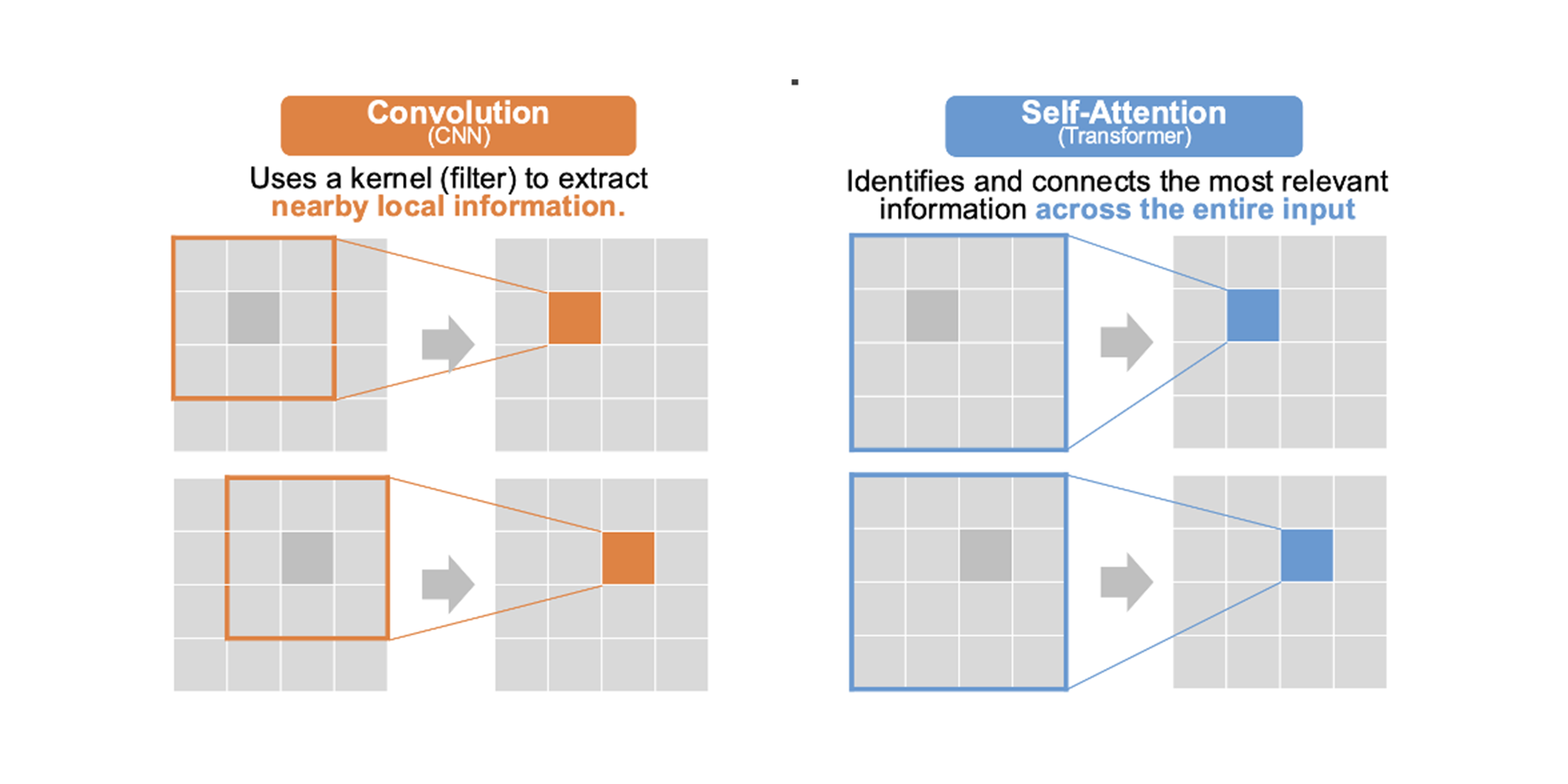
In 5G, channels are directly observed only at pilot REs; values at data REs must be inferred. Classical interpolators (e.g., LMMSE) or 2D CNNs rely on local neighborhoods and may underuse far-apart pilot information.
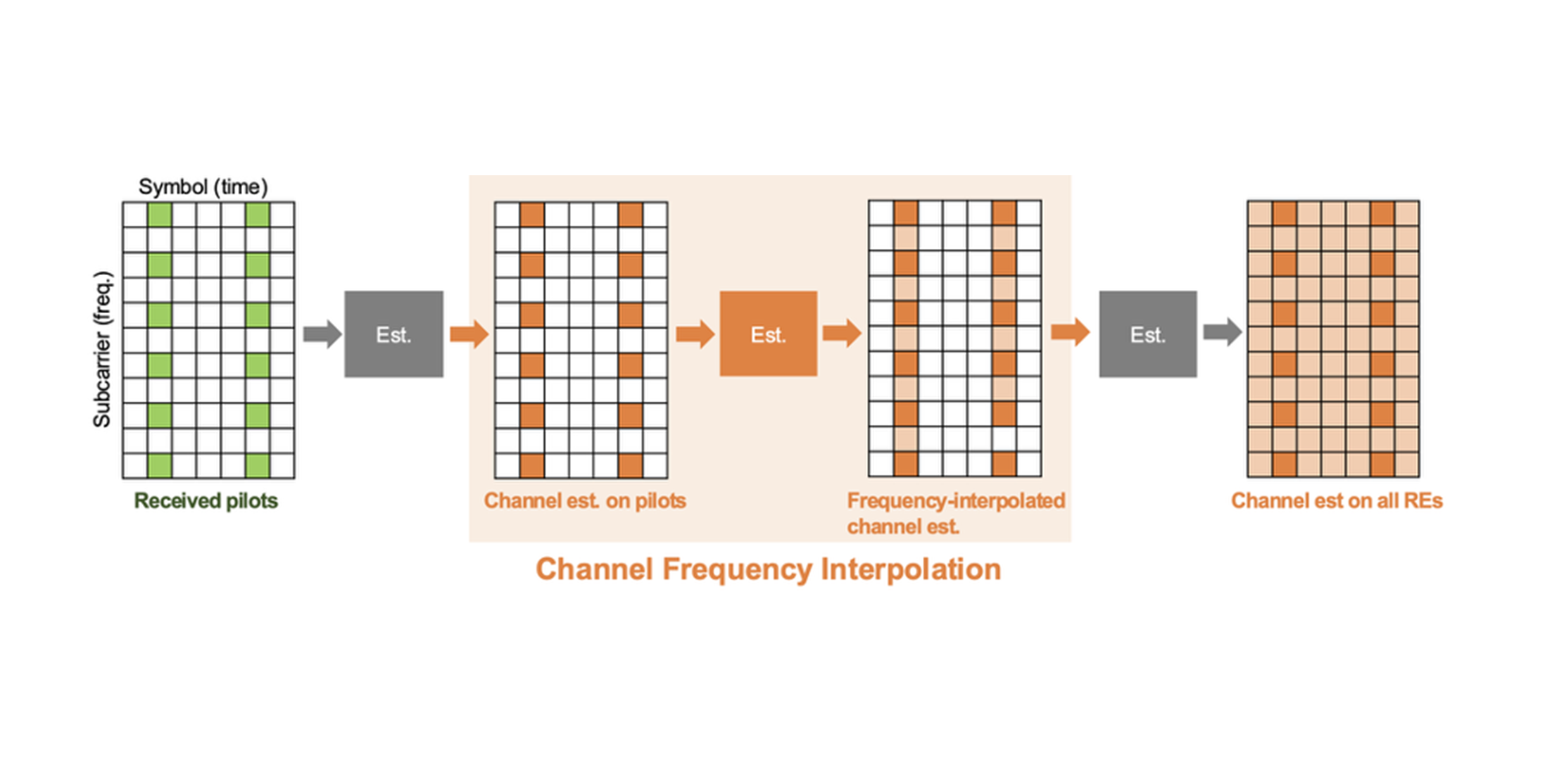
Fig. 4 — Channel-interpolation sketch: pilots (green) and predicted values at data REs (orange).
Approach
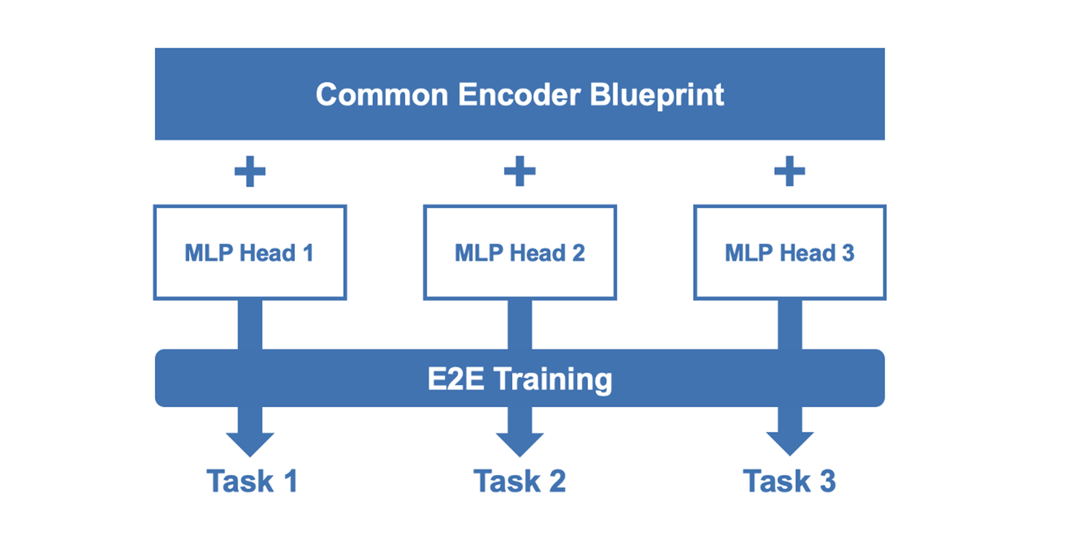
Instantiate the blueprint for interpolation: feed pilot estimates and a pilot mask; output a complex channel grid across the full band. Self-attention exploits long-range correlations across subcarriers and symbols that local kernels miss.
Results
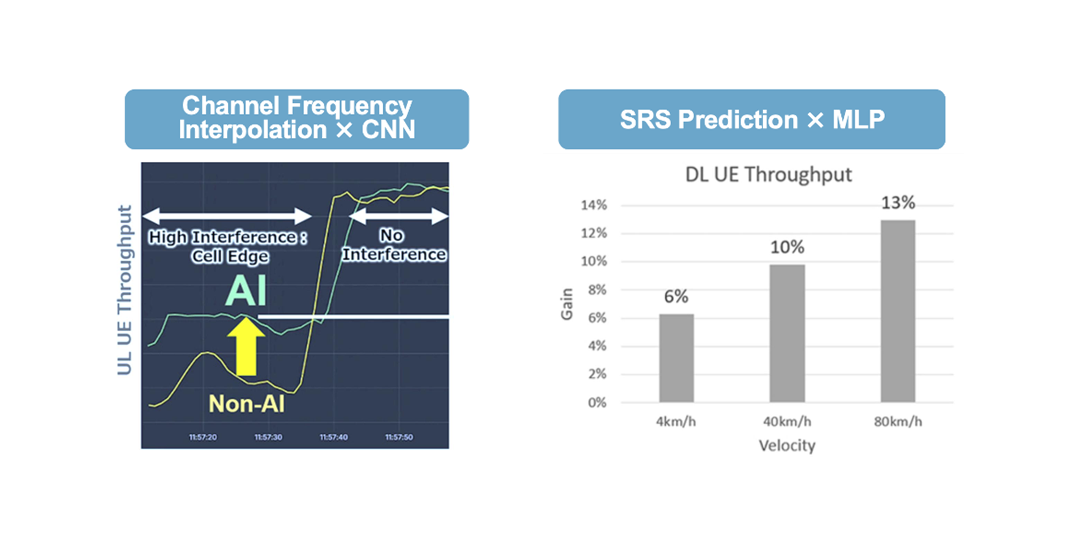
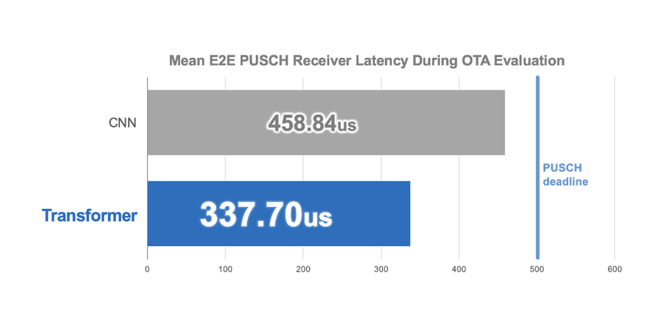
In 100 MHz n78 OTA evaluations, the Transformer interpolator achieved ≈ 30% uplink throughput gain vs LMMSE and ≈ 8% vs a CNN interpolator, with higher medians.
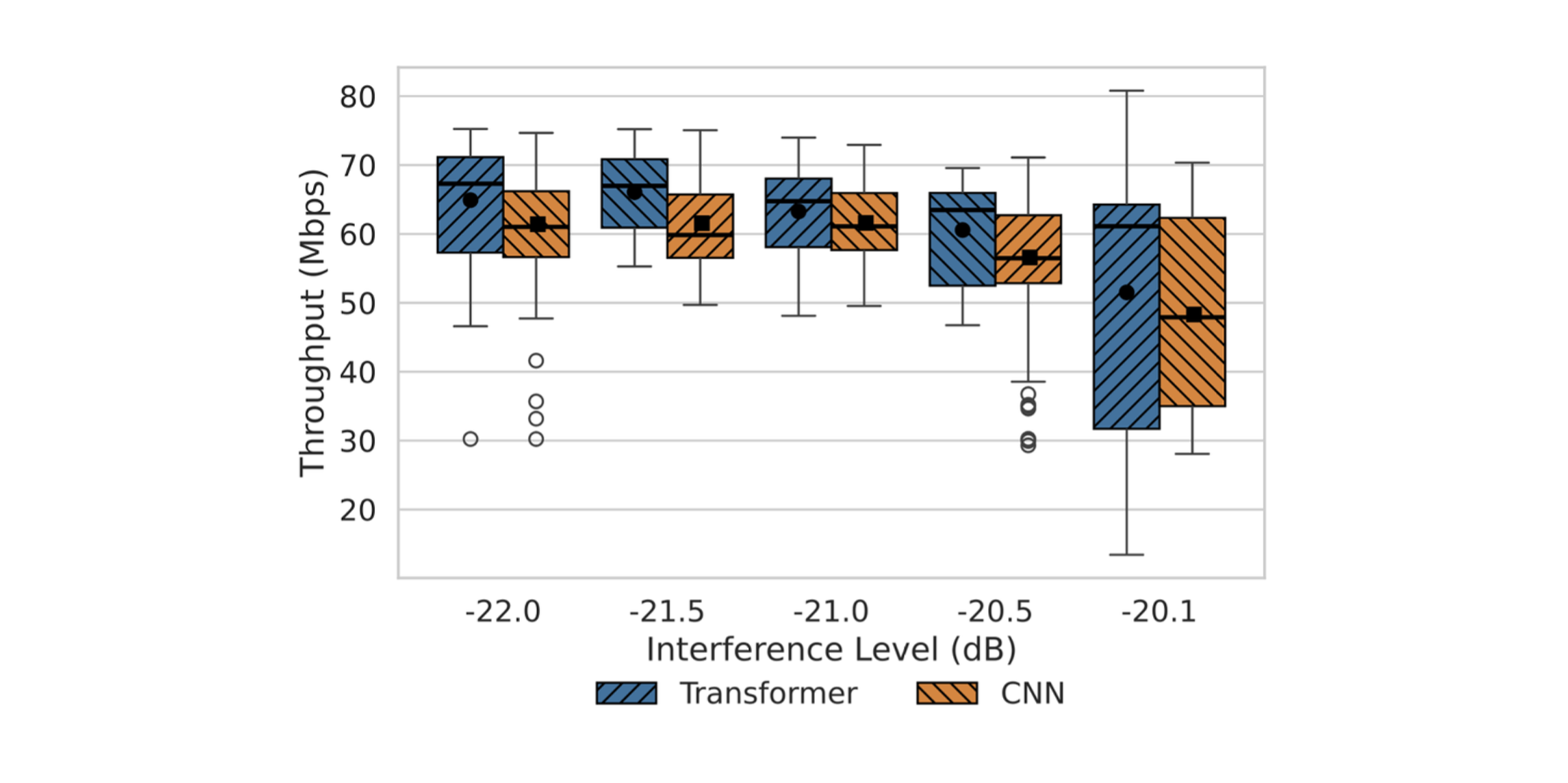
Fig. 5 — Uplink throughput (OTA): Transformer vs CNN vs LMMSE (box plots).
6.2 Sounding Reference Signal (SRS) Prediction
Problem
When uplink SRS reports are missing (UL gaps, mobility), the gNB must forecast near-future downlink beam quality to maintain alignment.
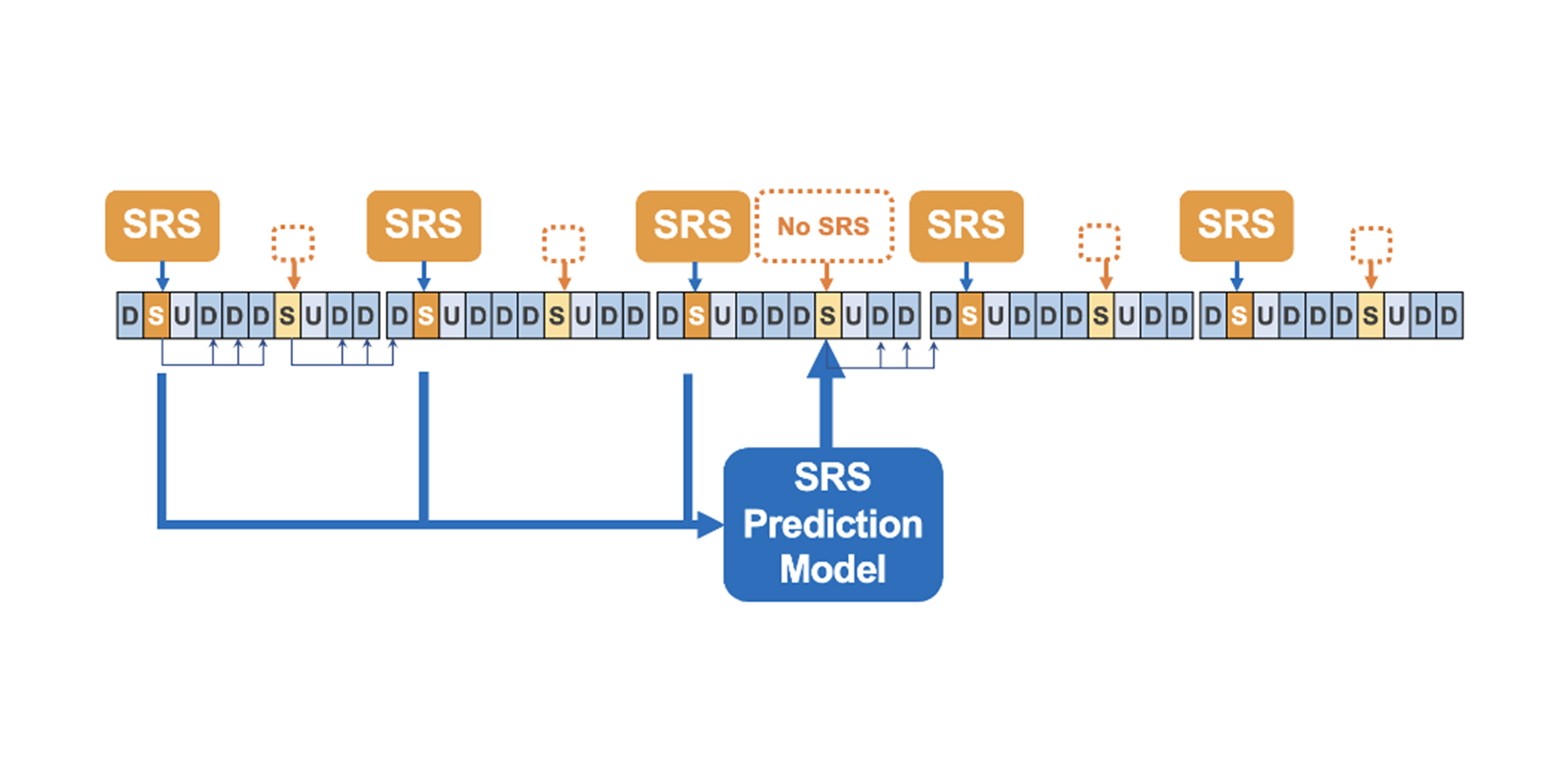
Fig. 6 — SRS prediction problem: missing SRS intervals on the UL timeline and the gNB’s forecast of the near-future channel.
Approach
Instantiate the blueprint for SRS prediction: ingest recent UL pilots/SRS and predict a future beam/quality for the target horizon. The global receptive field helps capture longer temporal dependencies.
Results
New simulations show ≈ 29% downlink gain at 80 km/h and ≈ 31% at 40 km/h, roughly 2.2–3.1× the gains of a prior MLP baseline.
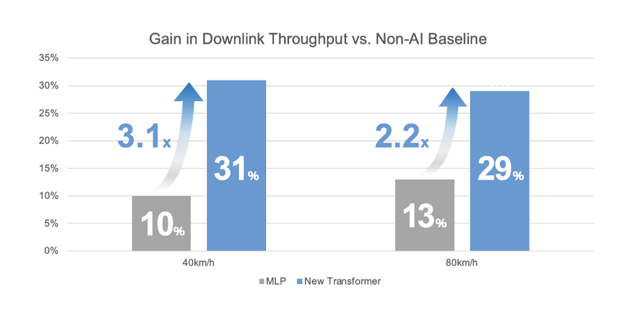
Fig. 7 — SRS prediction (simulation): Transformer vs MLP gains at 40/80 km/h.
7. Latency & Implementation
7.1 Meeting the 500 µs Deadline
Constraint
Uplink reception requires PHY processing in ≈ 500 µs.
Result
For 100 MHz PUSCH (OTA), the end-to-end receiver completes in ≈ 337 µs on NVIDIA GH200—≈ 1.36× faster than a CNN-based receiver—comfortably within budget.
Fig. 8 — Mean end-to-end PUSCH latency (OTA): Transformer vs CNN.
7.2 The GPU Imperative
Observation
Even lightweight models exceed the budget on CPUs alone (modern Xeon > 500µs).
Result
On NVIDIA H100, channel-interpolation inference runs in ≈ 0.205 ms, meeting the real-time target. GPUs (or dedicated AI accelerators) are therefore essential for practical deployment.
Fig. 9 — Inference time for channel interpolation: GPU (H100) vs CPU (Xeon).
8. Other Applications
End-to-end reception: Output LLRs directly to unify estimation → equalization → demapping, reducing BLER while respecting latency budgets.
Full-band channel estimation: Reconstruct the entire band from sparse pilots; observed to outperform CNN estimators.
Cross-layer hooks: Score user pairs for MU-pairing and other RRM tasks.
9. Challenges and Future Directions
Broader task coverage: Extend beyond interpolation/SRS to cross-layer functions (e.g., scheduling, resource allocation) so the blueprint contributes to end-to-end optimization.
Efficiency & scale: Refine positional encodings; apply compression and early-exit strategies to push the accuracy–latency–power frontier on baseband/edge hardware.
Robustness & evaluation: Improve behavior under high mobility/fast fading and advance 3GPP-compliant system-level evaluations.
Interpretability & standards: Use attention insights to inform pilot design and debugging while engaging with standards on the path from research to deployment.
10. Toward the Realization of AI-Native RAN
In this column we showed that attention-based signal processing can run over the air within slot-time constraints and that a reusable Transformer blueprint—RE tokenization, a shallow attention encoder, and task-specific (non-shared) heads—maps cleanly onto real RAN tasks. We illustrated the approach on channel-frequency interpolation (OTA) and SRS prediction (simulation) and discussed the practical pieces that matter in deployment: I/O conventions, runtime envelopes, and the need for accelerator-class inference.
From here, our focus is on broadening 3GPP-aligned evaluations, pushing efficiency (compression, early-exit, numerology-robust embeddings), and extending integrations toward scheduling and RRM. We’ll keep sharing what works—and what doesn’t—through papers, talks, and collaborations with partners who want to help build AI-native RAN.